Simulation Software Assists With Managing Mixed-Model Assembly
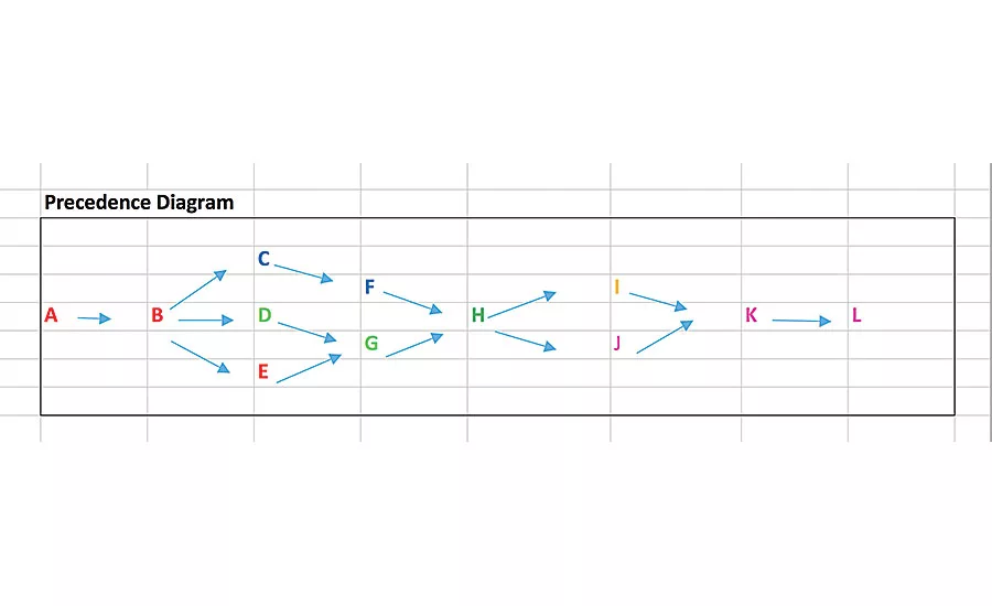
Fig. 1: Precedence Diagram. A precedence diagram is like a process flow diagram, with shapes and arrows describing the significant steps for assembling the product. Illustration courtesy Simul8 Corp.
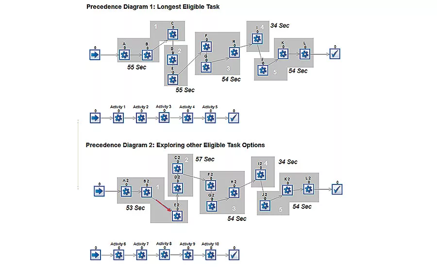
Fig. 2: Comparing Layouts. Simulation can help engineers compare precedence diagrams. These two precedence diagrams can be compared for number of units delivered. The first model (top) has greater capability, since it assembles 2,613 units vs. the second feasible layout, which assembles 2,521 units per week. Illustration courtesy Simul8 Corp.
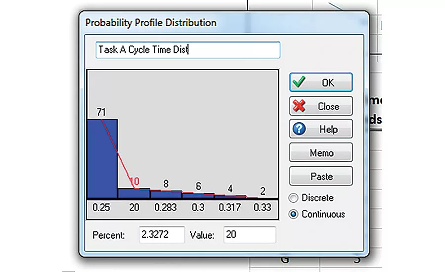
Simulation can examine the impact of tasks taking longer than normal. Here, a manual operation takes 15 seconds 70 percent of the time, but it takes 16 to 20 seconds 30 percent of the time. Illustration courtesy Simul8 Corp.
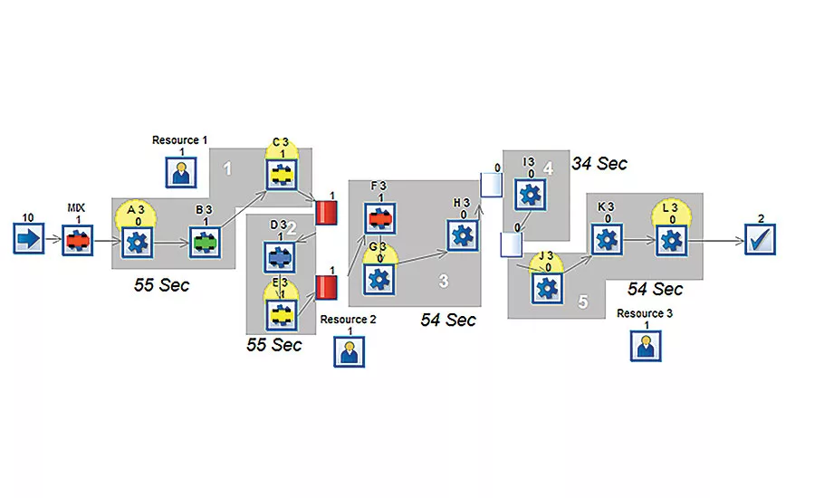
Using simulation, engineers can examine the impact of adding operators to a line. In this example, three operators cover six manual operations. The first operator handles tasks A and C at station 1. A second operator covers tasks E and G at stations 2 and 3. A third operator covers tasks J and L within station 5. In this scenario, throughput drops from 2,613 to 2,521. Illustration courtesy Simul8 Corp.
Simulation can be used to assess the effect of changeover and product mix on throughput. Illustration courtesy Simul8 Corp.
Line balancing is challenging, particularly when we are limited to approximations rather than exact data. With so many different and potentially conflicting requirements on the system, the outcomes of a new process design may be difficult to predict.
Simulation can create a well-balanced line that has the flexibility to hit throughput targets consistently. With a simple simulation of assembly operations on the line, we can identify bottlenecks, run different production schedules, and evaluate the impact of design and scheduling decisions, such as buffering requirements and product mix. This “what-if” analysis can be done quickly and accurately to evaluate all the conflicting decision criteria.
It’s About Time
When designing and managing a mixed-model assembly line, engineers strive to satisfy objectives such as maximizing throughput, minimizing the number of stations, balancing work across stations, satisfying delivery rates, and accommodating product mix changes. However, before we tackle these more complex objectives, we must first understand how many stations are required and how to assign tasks to those stations.
To determine how many stations are required, we start with a simple calculation derived from “takt time” and “total cycle time.”
Takt time is a calculation for what is required to meet demand: takt time = available working time / customer demand.
For example, let’s say our target is to produce 500 units per day within an 8-hour shift. Therefore, the takt time would be: 480 minutes / 500 units = 0.96 minute / unit = 57.6 seconds / unit.
To meet market demand of 500 units, each station must meet or beat that 57.6-second takt time.
Looking for quick answers on assembly and manufacturing topics? Try Ask ASM, our new smart AI search tool. Ask ASM
Next, we need to calculate total cycle time. This is the amount of time needed to produce a complete assembly from start to finish.
Let’s assume 12 steps are required to complete one assembly. Each step will have its own unique cycle time. These times can be measured with a stopwatch or estimated using MODAPTS. (MODAPTS, derived from “MODular Arrangement of Predetermined Time Standards,” is a standardized system for estimating how much time is needed to complete various manual assembly tasks.) To get the total cycle time, simply add the times for each step. (See “Calculating Total Cycle Time” table on pg. 39.) In our example, total cycle time is 252 seconds.
The required number of stations can now be calculated: number of stations = total cycle time / takt time. In our example, the number of stations would therefore be: 57.6 / 252 = 4.46, or 5.
Assigning Tasks to Stations
Now that we know 12 tasks must be accomplished within five stations, it becomes a question of which tasks to include at each station. To do that, we need to list the processes for assembling the product and the order in which they are accomplished. The list should clearly indicate which steps must be done synchronously and which can be done simultaneously.
This can be captured in a precedence diagram. A precedence diagram is like a process flow diagram, with shapes and arrows describing the significant steps for assembling the product.
Figure 1 shows the precedence diagram for our example. The diagram clearly shows that task A must be completed before task B can be started. It also shows that that tasks C, D, and E can be started simultaneously after task B has been completed. Moreover, both tasks F and G must be completed before task H can start.
We can now add a precedence column to our initial task table. (See “Taking Precedence” table, right.)
We can now start assigning tasks to stations. One common approach is to use a task assignment table. (See “Task Assignment” table on pg. 41.) This table looks at all eligible tasks to be included within a station, and keeps track of the accumulated cycle time within the station. A common scheme is to start in the order of the precedence diagram and seek the longest cycle time.
Remember, we have five stations and each station has 57.6 seconds to play with.
We start with Station 1. The only eligible task is Task A, so Station 1 gets Task A and its 15-second cycle time. The remaining time left within the station is the takt time minus the assigned task (57.6 seconds – 15 seconds = 42.6 seconds). Therefore, we have 42.6 seconds remaining in Station 1 for additional tasks. The only qualified task is Task B, so we can add that task to Station 1, as well.
We now have a remaining time of 19.6 seconds. The next tasks are C, D, and E. Task D won’t work, because its cycle time is greater than the time left at that station. Since we are using the longest cycle time rule, we will assign Task C (17 seconds) to Station 1, too.
Station 1 is now full. No more processes can be added, since none of the remaining tasks take less than 2.6 seconds to complete.
We are now ready to assign tasks to the second station. The eligible tasks are D and E. Since D has a higher cycle time of 42 seconds, it will be the first task assigned to Station 2. Adding Task E (15 seconds) fills this station. The remaining idle time is just 0.6 second.
The remaining three stations can then be completed in the same manner. Although Station 4 is under-cycle with 23.6 seconds of idle time, this layout would seem to be the best available setup according to the process precedence rules.
Going Beyond With Simulation
These tables and diagrams offer a lot of insight into laying out an assembly line. However, when this information is coupled with simulation analysis, engineers can go vastly beyond these simple calculations.
All of our earlier charts and calculations assume no random downtime, over-cycles (a task taking longer than normal), changeovers, or other issues. They also do not consider shared operators capable of working on various tasks. If we try to bring these variations into our analysis, the calculations become very complex. With simulation, these parameters are handled with ease.
Simulation can easily be applied at the start of your precedence diagrams. This is a natural starting point, since they depict the process steps and routing links. Each diagram can be modeled, and all eligible routing variations can be compared by simply changing routing links. These small models are initially done at the task level, once the best precedence diagram scheme has been proven. Later, they can be rolled-up and modeled at the station level to look at cycle times.
Figure 2 shows two precedence diagrams that can be compared for number of units delivered. Remember, our original target was to achieve a minimum of 500 units per shift or 2,500 units per week. We can clearly see that the first model has more capability, since it can assemble 2,613 units vs. the second feasible layout, which can assemble 2,521 units per week.
Adding Operators
A common consideration is what happens when manual operations are added to a precedence diagram. This is easily accomplished with simulation. Returning to our example, let’s consider that tasks A, C, E, G, J and L are manual operations. All of the other operations are automated.
Typical questions that arise include:
- How many operators are required?
- What impact do they have on throughput?
- Can the target of 500 units per shift be met with three operators?
- Which operator is potentially causing losses?
All these questions can be answered with simulation by testing various operator schemes. Simulations can even include travel time between stations.
Through simulation of our example line, we placed three operators to cover the six manual operations. The first operator handles tasks A and C of station 1. A second operator covers tasks E and G, which are at different stations. This operator requires additional travel time to walk between stations 2 and 3. A third operator covers tasks J and L within station 5. In this scenario, the overall number of units produced has dropped from 2,613 to 2,521, which is slightly above the target.
From the analysis, we can determine that the shared resource between station 2 and 3 is causing the slight loss in throughput. While this layout could be considered within our design specifications, it could also be a potential trouble spot. If unexpected events occur, such as downtime or changeovers, there could be significant losses.
This is a very common scenario. Most companies strive to keep their workforce to a minimum and achieve a high utilization per operator. Simulation offers great insight into the optimal placement of operators for achieving resource utilization targets and balancing workloads.
Accounting for Over-Cycles
Simulation can also look at over-cycles. Returning to our imaginary assembly line, let’s assume any of the manual operations can experience up to a 5-second over-cycle 30 percent of the time. In other words, task A, for example, will take 15 seconds 70 percent of the time; but it will take 16 to 20 seconds 30 percent of the time. This is known as a probability profile distribution.
Using simulation, we can place this type of distribution on the remaining manual operations. When we crunch the numbers, we find that our line produces 2,472 units per week, which falls below the targeted throughput by 28 units.
Accounting for Downtime
We can also add downtime to the simulation by applying data for “mean time between failures” (MTBF) and “mean time to repair” (MTR). For example, all of the automated tasks might be 95 percent efficient, with an MTBF of 90 minutes and an MTR of 5 minutes.
When we run the previous scenario with the additional downtime on all of the automated tasks, throughput drops significantly to 1,777 units per week.
This is where more advanced line balancing techniques are required.
Let’s go back to station 1, which accomplishes tasks A, B and C. Tasks A and C require an operator, and task B is automated. What if task A can be started while task B is cycling? As you can imagine, there are many scenarios that could be built into the process steps of station 1. Station 1 could have an input buffer and an output buffer, commonly referred to as “decouplers.” These minimize the losses related to sequential downtime on synchronous stations. Evaluating any of these line-design scenarios would be difficult without simulation.
Mixing It Up
Finally, simulation can examine the impact of changeovers. Many assembly lines today produce a mix of products. These product variations might be assembled in batches or at completely random intervals. Either way, this adds great complexity to line balancing, since each station may have unique cycle times depending on what it’s producing. Changeover time also needs to be considered. Tooling might need to be swapped. Process parameters might need to be changed.
With simulation, it’s easy to account for such changes. For example, let’s say an automotive assembly line produces the same vehicle in four colors (28 percent blue, 34 percent red, 9 percent green, and 29 percent yellow). Changeover between colors takes 2 minutes.
This scenario would more than likely require a batch-build scheme to minimize the number of changeovers. One scheme would be to group the daily orders of 500 units in four groups, by color. This would reduce the average number of changeovers to four per shift.
Looking for a reprint of this article?
From high-res PDFs to custom plaques, order your copy today!