Monitoring Activity During Wire Harness Assembly
New technology helps engineers gather real-time data on manual assembly processes, such as wire harness assembly.
Industry 4.0 and the digital manufacturing revolution are all about collecting—and, more importantly, acting on—data gathered from the assembly process in real time. That’s all well and good when data is coming from sensors, vision systems, fastening tools and other electronic devices. But, how can engineers gather real-time data on largely manual assembly processes, such as wire harness assembly?
To solve this problem, we developed a software- and sensor-based system to measure activity times and performance on a wire harness assembly line. To ensure a real-time connection between assembler performance and varying product complexity, our system relies on fixture sensors and an indoor positioning system (IPS). Our goal was to create a system that could continuously estimate the time consumed by the various elementary activities that make up wire harness assembly. Our system creates a model of a task, compares estimated activity times to the actual performance of assemblers, and generates early warnings when their productivity decreases.
To reliably and cost-effectively measure assembly times, we developed sensors that begin timing an activity when an assembler inserts a component into a fixture. Since the activities of assemblers depend on the type and number of built-in components, production flow is tracked by the IPS. To localize assemblies and identify the status of the conveyor system, we used ultra-wide band IPS technology, due to its low energy demand for transmitting information over a broad bandwidth (more 500 megahertz) and its ability to locate an object with an accuracy of 30 to 50 centimeters. (That is significantly better than the 1-meter accuracy of Bluetooth low-energy-based systems.)
To integrate measurements originating from the IPS, we integrated a varying number (10 to 100) of active or passive fixture sensors and other information sources, and we developed a multisensor data fusion algorithm. Multiple sensors provide redundancy, enabling the robust recursive estimation of unmeasured primary activity times of the assemblers. To constrain the model parameters to lie within a reliable region and incorporate important a priori knowledge concerning activity times, the estimated parameters were optimally projected on to a set of linear constraints by quadratic programming. This central estimation enhances the confidence of the nominal model, which improves the performance of fault detection based on the reconciliation of local measurements.
To ensure our results are fully reproducible, only openly available information on wire harness manufacturing technologies was used during the development of our case study. To stimulate further research, the algorithm of our model of the manufacturing system and the details of the products and sensor placements are publicly available on our website: https://www.abonyilab.com/soft-sensors.
Our Model
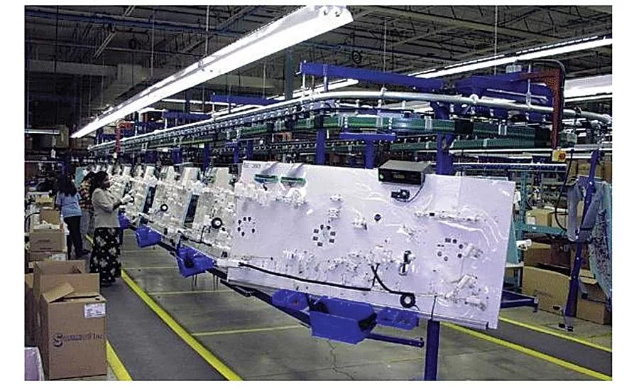
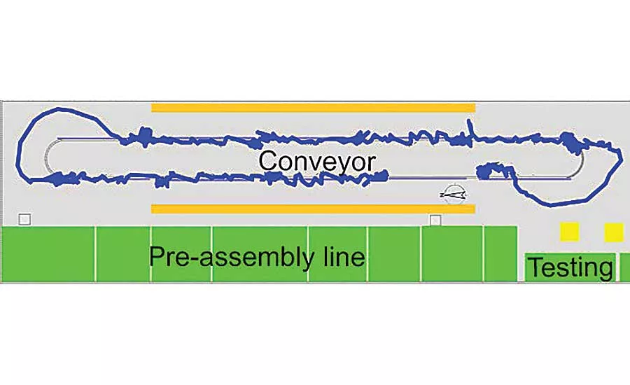
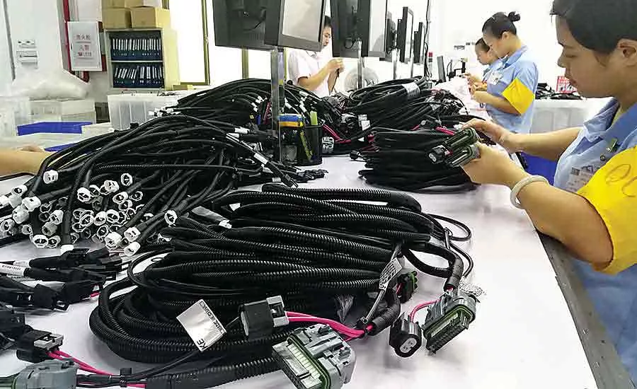
For our study, we looked at high-volume production of a large, complex wiring harness for a motor vehicle. Harness assembly boards are hung from an overhead conveyor. The motion of the conveyor is paced and cyclic. The line operates according to an open-station concept. When an assembler does not finish his job, he can move with the product to the next station to reduce the backlog. When the assembler completes the task before the end of the allotted cycle time, he can work ahead of schedule. Production stops when the delay exceeds a critical limit. (In contrast, in a closed-station operating concept, the assembler must stop the conveyor even in the event of a minor delay.)
Expected activity times are estimated based on the bill of materials of the harness. Manufacturing is modular, meaning that the products (p1, p2…pNp) are built from the set of modules (m1, m2…mNm). The structures of the products are defined by a P-matrix, consisting of Np rows and Nm columns, and the element pi,j of P is set to one when a pi product contains an mj module (otherwise it is 0). The calculation of the theoretical activity times is estimated based on which activities (a1, a2…aNa) need to be performed and which components (c1, c2…cNc) should be assembled at which workstations (w1, w2…wNw).
Looking for quick answers on assembly and manufacturing topics? Try Ask ASM, our new smart AI search tool. Ask ASM
This information is represented in the logical matrix M that contains the activities required to produce a given product. As shown in table 1, the C matrix stores which components are assembled during each activity, while the W matrix assigns activities to the workstations. The specific activity times and the factors influencing them were determined based on expert knowledge, as presented in table 2. The T matrix provides information on the category of the activity, describing how the activities are classified into the activity types (t1, t2…tNt). The sequence of the products is represented by a π vector of the labels of the types, so π (k) = pj states that product pj started to be produced during production cycle k.
For our study, the number of types of products Np is assumed to be 64 and defined as the combination of seven modules: the base module m1, left- or right-hand drive m2, normal or hybrid m3, halogen or LED lights m4, gas or diesel engine m5, four doors or five doors m6, and manual or automatic gearbox m7. The number of activities Na is defined as 654 and categorized into 16 types. The time consumptions of these activities are approximated using a direct proportionality approach with regard to the primary activities. During the activities involved in the production of the base harness, 115 component types Nc are assembled. These include Ct (162 terminals), Cb (63 tape wraps), Cc (25 clips) and Cw (89 wires). The conveyor consists of 10 workstations, each of which is staffed by one assembler.
The term primary activity time denotes the estimated average time required for a certain type of activity to be performed, while the term local activity time refers to the time required by a specific assembler at a specific workstation to perform the activity in question.
Our proposed matrix-based mathematical formulation is beneficial, as it allows the compact estimation of the individual activity times in each cycle step: Ŷiw(k) = [ti, ci] xw(k). The time consumption of the i activity depends on how many elementary activities of a given type should be performed (represented as ti, which is the i row of the matrix T), the number of built in components (the row vector ci is the i row of the matrix C) and the efficiency of the assembler xw(k), which is the vector of the estimated local activity times. Therefore, the aim of our investigation was to provide a continuous local estimate of this state vector and its workstation independent x(k) version, providing a reference value and the opportunity for the isolation of assembler-independent problems.
Time Measurements
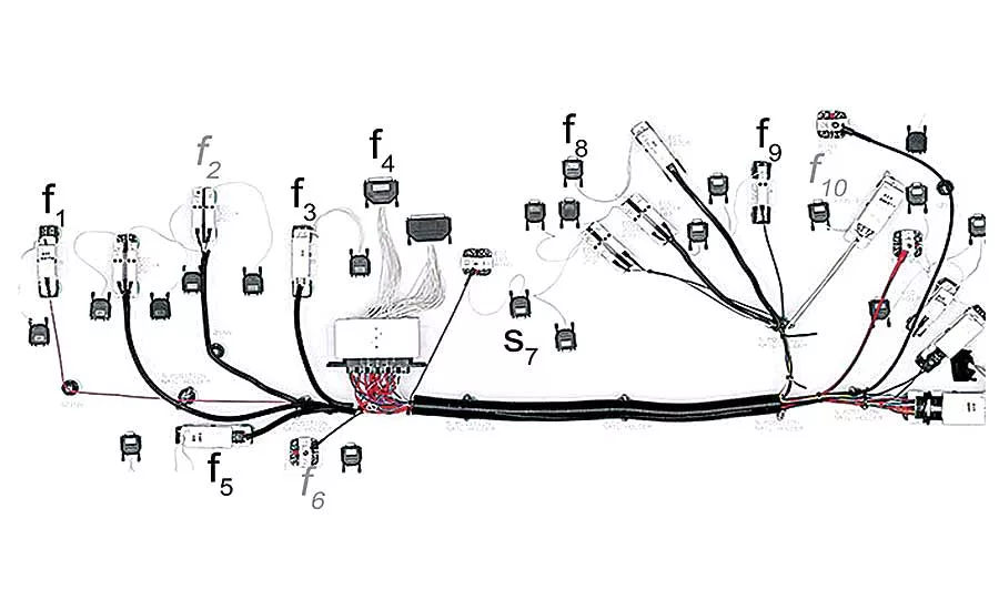
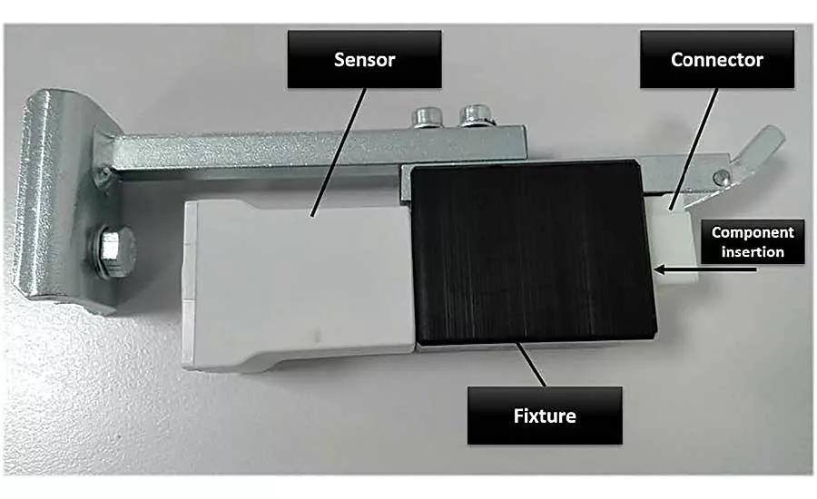
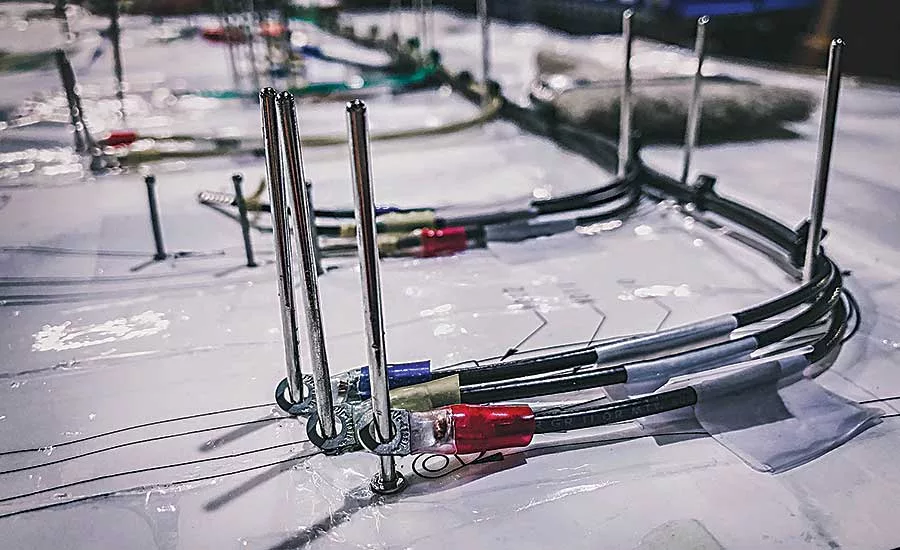
To measure the activity times, we designed fixture-based activity sensors. These sensors generate time stamps when a component is inserted into the fixture.
The fixtures were positioned based on how the measurable activities at the workstations are distributed. For example, the sensor f1 sends a time stamps when the assembler inserts the component c1, which represents the starting time of the first activity a1.
The activity-dependent sequence of time stamps recorded by the active sensors in the k cycle of the conveyor is represented by vector s(k) = [s1(k)…sj(k)…sNs(k)]T, which serves as the raw input of the performance-monitoring algorithm.
Any two time stamps clasp a set of activities. Therefore, the ziw(k) = sβ(i)w(k) ̶ sα(i)w(k) difference between any two time stamps provides the sum of the activity times that are situated between the two sensors. If the time stamps sα(i)w(k) measures the start of the first activity at the w workstation, the station time at that workstation can be measured as ziw(k) = sα(i)w(k + 1) ̶ sα(i)w(k). Based on this concept, a set of measurements can be defined for the workstations ziw(k) = [z1w(k)…ziw(k)…zlww(k)]T, which is much more interpretable and applicable information with regard to activity-time monitoring than the s(k) values of the raw measurements.
To put zw(k) into context, the information on which products are assembled at each station and the details of the activities that are assigned to the measured time interval ziw(k) are required.
The assignment of the activities and the measured time intervals are represented by a set of logical matrices Sw (see table 1). In the case of modular production, the set of activities qa = MppT should be calculated based on which modules are included in the produced p-th product (represented as pp which is the p row of the product-module matrix P) and whose activities are required to produce the modules (such information is stored in the relation matrix M). The activities that are assigned to the ziw(k) intervals are defined by the operation diag(qa)Sw.
TTdiag(qa)Sw groups the activities according to activity types, while the number of components installed over a specific time interval is calculated as CTdiag(qa)Sw, which can also be grouped by activity types according to (TTC > 0) CTdiag(qa)Sw. Based on the proposed matrix-type representation, the estimated time intervals at the w workstation can be calculated as: zw(k) = [TTdiag(qa)Sw, (TTC > 0) CTdiag(qa)Sw] xw(k) = Hw(k)xw(k).
The model equation zw(k) = Hw(k)xw(k) + ew and the related measurements zw(k) can be used for the continuous estimation of the vector of assembler efficiencies (namely, estimated local activity times), xw(k), where ew(k) is assumed to be a serially uncorrelated white-noise vector of observational errors with covariance matrix Rw(k).
As Hw(k) depends on the actual product, which product is produced at the w workstation must be tracked. For the localization of products and identification of the status of the conveyor system, IPS technology was applied.
Compared with outdoor environments, sensing location information in indoor environments requires higher precision, which is a more challenging task because various objects reflect and disperse signals. UWB is an emerging technology in the field of indoor positioning that has shown better performance compared with others. Depending on the positioning technique, the angle of arrival, the signal strength or time delay information can be used for positioning. Received signal strength positioning methods can also be divided into time of arrival, angle of arrival and received signal strength-based systems.
The concept of identification products at workstations to extract information from the bill of materials and other structured information sources is widely used to support production management, value stream mapping, and Industrial Internet of Things projects. In our system, the IPS beacons are mounted to the flat wire harness, and the raw signals of the receivers are processed to assign the cables to the workstations.
Fusion-Based Recursive Estimation
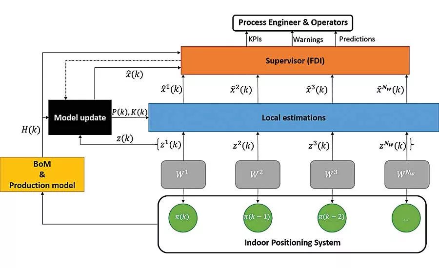
Multiple sensors provide redundancy, which enables robust recursive estimation of the unmeasured primary activity times of the assemblers. Therefore, the estimation problem is defined as a sensor-fusion task. Our sensor fusion algorithm combines all sensory and production data, such that the estimates of the activity times have less uncertainty than would be possible when these sources were used individually. The elements of the monitoring system are structured as shown in Figure 6.
The fusion center receives and synchronizes all the measured time intervals and the related time-variable regressors, which means all data collected from the workstations are time-stamped and arranged according to k cycle of the conveyor: z(k) = [z1(k)…zNw(k)], H(k) = [H1(k)…HNw(k)].
The linear structure of our production-monitoring model is adequate for our analysis, as the time consumption of the activities linearly depend on how many elementary activities should be performed and how many components must be assembled. When a linear sensor-fusion model is assumed, the linear time-variant model can be represented as z(k) = H(k)x(k) + e(k), where the e(k) noise vector of the fused observations consists of the ew(k) serially uncorrelated white-noise vectors of observational errors at the workstations, e(k) = [(e1(k))T…(eNw(k))T]T.
When the observation errors of the workstations are assumed to be independent, the covariance of the e(k) noise vector is a block diagonal matrix defined as R = diag(R1…RNw).
The central estimation enhances the confidence of the nominal model, which improves the performance of fault detection based on the reconciliation of the local measurements.
Wire Harness Case Study
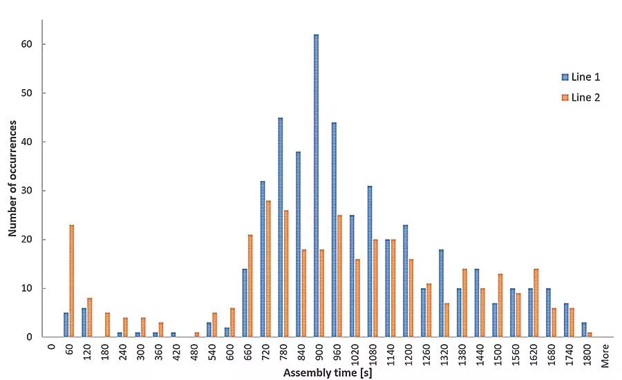
To validate the reliability of the proposed model, we studied the distribution of activity times collected from real production lines. Histograms of the data indicate that the distribution of sensor-delivered processing times can be decomposed into normal distribution functions.
When only one product is produced, H(k) does not change in terms of time. In this case, the set of identifiable parameters for a given product can be determined by the QR decomposition of H(k) (or Hw(k) when a local estimation is needed). When different products are produced, the variation in H(k) significantly increases the available information, so the optimization of the production sequence can highly influence the ability of the model to identify problems.
Production of 1,000 harnesses was studied. The production sequence contained all 64 types of products with an average batch size of 10 products.
When the raw material, design or the processing of a component in a cost-cutting or quality-improvement project is changed by the supplier, this change may influence the activity times of the assemblers. Such assembler-independent loss in performance can occur when a shorter length of wire increases the time required to lay and arrange the cables.
In our case study, such effects were monitored. New wires between the c87 and c8 components were introduced, and they were a bit shorter than specified. The component c87 (seal on the terminal) affects activity t10 in the module m4, which increases the related primary activity time x10(k) by 15 percent at the 200th product, while the component c8 (the shorter wire) affects activity t5 in module m2, which increases the related primary activity time x5(k) by 20 percent after the 300th product. However, quality inspection time decreases after the 500th product.
Our system is able to track both the slowed and quickened activities. The benefit of our constrained algorithm is clearly visible: The estimated variables converge faster and are always reliable.
We also looked at ways of detecting individual losses in assembler performance and sensor faults (due to delayed registration and Internet communication).
In terms of fault detection, our algorithms can be used to generate an interpretable and easily traceable univariate time series that reflects the global performance of the model. The global performance of the model is reflected by eq(k) = [z(k) ̶ H(k)x]T Q[z(k) ̶ H(k)x].
Based on the analysis with regard to the rank of the Hw(k) matrices, observable sets of activities were determined. For example, at workstation 2, the time consumption of six primary activities was observable. Our algorithm was able to detect assembler-dependent problems related to those activities. What’s more, by monitoring the eq(k), it was possible to determine when sensor faults occurred. The parameters of the gross error detection algorithm can be fine-tuned by Monte Carlo simulation and detailed analysis of the distribution of the modeling error.
Our calculations can also be used to estimate the expectable operation times for all workstations, check how well the process is balanced, and how the complexity of the product influences the workloads of the workstations. With our model, the effect of changes in activity time can be immediately calculated on the takt time and effectiveness of the assemblers. With good estimates of the duration of primary activities, and with the help of IIoT-based fusion of product-relevant information, real-time data for overall equipment effectiveness calculations can be provided.
Model-Based Workload Analysis
Monitoring the activity of assemblers is based on the comparison of the measured activity and station times with the estimates of targeting models. Targeting models are widely used in process performance management. Precedent-based targeting models are used when the expected performance can be deduced from previous operations (for example, a day or month before). One weakness of this procedure is that it assumes that conditions were comparable over the two time intervals. A more problematic issue is what happens when a significant change occurs in the process and product. For such applications, precedent-based targeting models can be over simplistic. Activity-based targeting is particularly appropriate when the clear drivers of performance are known.
Automatic monitoring and targeting schemes attempt to compare performances very short time intervals (minutes), which is ideal for fault detection. The most important key performance indicators of the production system are the station times, which reflect how well the production line is balanced.
Balancing a modular production system is a challenging industrial problem, due to the great diversity of products. As the station times are the functions of the manufactured products, which product is assembled on a given workstation must be followed. The calculation of the station time is similar to the calculation of the estimated sum of activity times between two fixture sensors—namely the difference between the time stamps recorded by the fixture sensors.
Table 1: Logical Matrices for Performance Monitoring
| Notation | Nodes | Description | Size |
| A | product (p) - activity (a) | activity required to produce a product | Np x Na |
| W | activity (a) - workstation (w) | workstation assigned for an activity | Na x Nw |
| B | product (p) - component (c) | component/part required to produce a product | Np x Nc |
| P | product (p) - module (m) | module/part family required to produce a product | Np x Nm |
| C | activity (a) - component (c) | component/part built in or processed in an activity | Na x Nc |
| M | activity (a) - module (m) | activity required to produce a module | Na x Nm |
| T | activity (a) - activity type (t) | category of the activity | Na x Nt |
| Sw | activity (a) - measured time interval (zw(k)) | activity involved over a measured time interval | Na x lw |
Table 2. Types of Harness Assembly Activities and Their Times
| ID | Activity | Time (seconds) |
| t1 | Point-to-point wiring on chassis | 4.6 |
| t2 | Laying in U-channel | 4.4 |
| t3 | Laying flat cable | 7.7 |
| t4 | Laying wires onto harness jig | 6.9 |
| t5 | Laying cable connector (one end) onto harness jig | 7.4 |
| t6 | Spot-tying cables and cutting ends | 16.6 |
| t7 | Lacing activity | 1.5 |
| t8 | Taping activity | 6.8 |
| t9 | Inserting into tube or sleeve | 3 |
| t10 | Attachment of wire terminal | 22.8 |
| t11 | Screw fastening of terminal | 17.1 |
| t12 | Screw-and-nut fastening of terminal | 24.7 |
| t13 | Circular connector | 11.3 |
| t14 | Rectangular connector | 24 |
| t15 | Clip installation | 8 |
| t16 | Visual testing | 120 |
Looking for a reprint of this article?
From high-res PDFs to custom plaques, order your copy today!