Like any other electric motor, a permanent magnet electric motor works on electromagnetic principles and has some mechanical function to perform at every instance of its operation. With increasing demand for more compact power density in miniature motors, the establishment of useful life and the methodology to establish that life becomes important for motor manufacturers or engineers.

Let’s first review the way to predict the life of such permanent magnet motors, using a Weibull diagram and reliability fundamentals.  Based on a complex mathematical model, the Weibull diagram allows estimating the expected life of a motor by measuring a few samples.  This can better help understand the process used to estimate motor life in an application.

The Motor Basic Torque Speed Curve

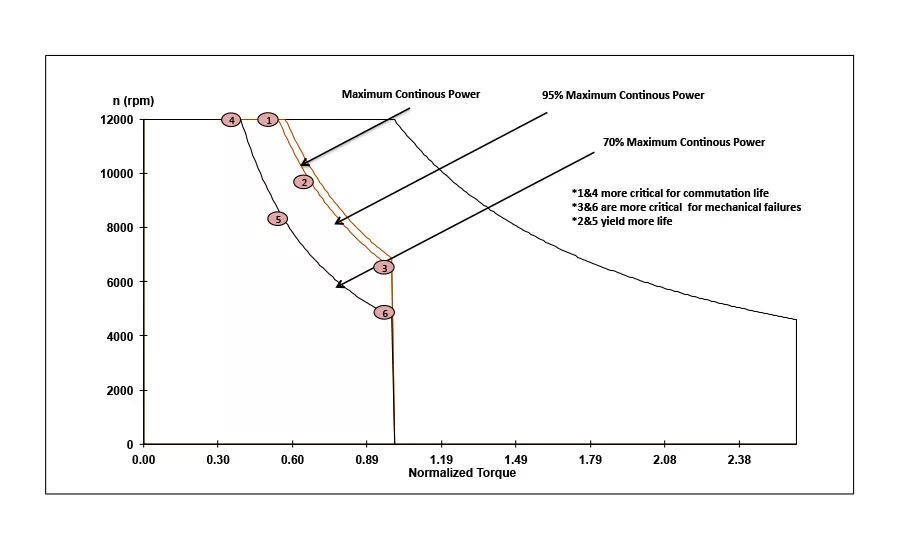
The Characteristics of motor is represented by its speed torque characteristics. Below is the graph (Figure 1) of DC motor with precious metal commutation that shows torque on X axis and Speed on Y axis. 

The maximum continuous torque line marks the thermal limit of using the motor continually without overheating the motor in normal conditions. The region on the right and left side of the maximum continuous torque line are called intermittent and continuous operating zones. In intermittent region the motor can be operated for a short duration that depends on how far it is operating from maximum continuous torque line. The farther the motor is operating; shorter will be the duration of its operation at that working point.

The critical motor design factors defining reliability at various working points is also defined in Figure 1.  Reliability at the high speed working points (point 1 and point 4) is function of commutation and bearing design.  Reliability at maximum continuous torque working points (point 3 and point 6) is a function of its thermal design. Reliability at any working point on right side of maximum continuous torque line is function of both thermal and mechanical design. The curve line shown by points 1-2-3 shows 95% of maximum continuous power and point 4-5-6 shows the 70% of maximum continuous power curve.  Operating at 70% of maximum continuous power will have higher reliability than operating at 95% of maximum continuous power curve.

The Seven-step Methodology for Estimating Reliability

Increasing higher speed requirements from a permanent magnet miniature DC motor is increasing stress on its commutation system design or bearing design whereas increasing high torque requirement increases stress on its thermal and mechanical design of various subassemblies. This signifies that the reliability of the motor varies if we operate a DC permanent magnet motor at Point 1 Vs at Point 2 Vs at Point 3 as explained above and shown (Figure 1). 

In order to understand the reliability of motor at these different working points, one needs to perform seven steps methodology as shown below:

1. Identifying application requirements

a. It is extremely important to understand the application working point and cycle (i.e. Torque-Speed requirements over time with direction of rotation), the environment in which the application is operating (i.e. temperature and humidity), and life expectancy of the application or motor under discussion. For target life, most equipment manufacturers who use a motor as a driver in their application are well-versed with the life of the product they are developing. The target life of a motor is a function of this expected life of the product. 

2. Identifying test equipment to simulate the application

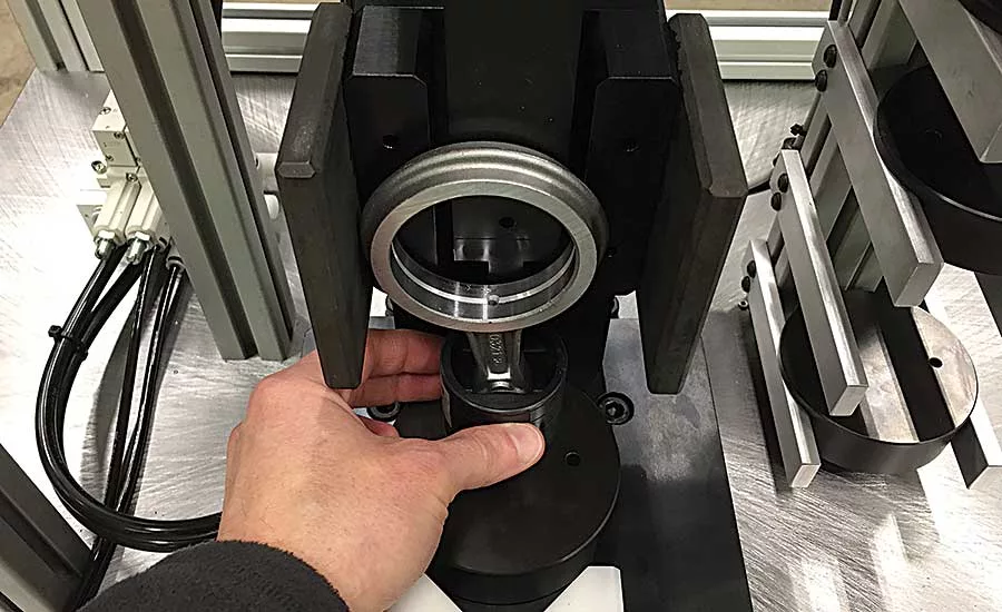
a. This is a difficult task for motor manufacturers as they mostly do not have the real application setup. The application torque-speed-time requirement helps the reliability engineer or motor designer to test motors that will nearly replicate the actual application setup. In such conditions, a simple motor can be mounted on a fixture and loaded with an eddy current or electromagnetic brake, or a function generator. The purpose of these brakes is to apply constant torque on the motor output shaft. A function generator generates the required torque-speed-time characteristics and loads the motor accordingly. This simple setup can be kept in an environmental chamber where application temperature and humidity conditions can also be applied.

3. Identifying the number of motors to be tested and each working point

a. The number of motors at each application point (Torque-Speed point) may vary from 5 to 30 depending on availability of motors, accuracy of data required and the nature of the testing facility available in reliability lab. As a general rule, if more motors are tested, the confidence on the life predicted or reliability increases, as we have more data points or continuous data that represents the population of motors being tested.

b. The working point should cover high speed-low torque point (Figure 1 - Point 1) and low speed-high torque point (Figure 1 - Point 3). Life expectancy at these working points may be low as these are extreme points for commutation or thermal / mechanical failure of the motor. These points define limits of life during continuous operation of a motor. The life at mid torque and speed is higher and provides the useful life. 

4. Reliability Testing & Weibull Curve

a. The next step is to perform reliability test of each motor at the defined working points, cycle and environment conditions. The motors can fail at any time depending on its design. The failure is usually visible by increase in current drawn, overheating or mechanical failure. Therefore it is very important for a reliability engineer to keep measuring these parameters continuously during reliability testing. Once target motor life is achieved, the motors that are still running can continue to run until end of their life to understand the actual life of the motor.

b. Weibull distribution is widely used for life prediction, since it is a generic distribution which encompasses exponential, normal, and other distributions. Simply speaking, a Weibull distribution represents a line where the Y axis represents the failure rate or unreliability and the X axis represents the time to failure. The slope of this distribution or line is called the shape parameter (b ). The intercept of this line with X axis is used to calculate scale parameter or characteristics life ( h). The characteristics life is life at 63.2% of failure. The intercept of the Weibull plot on x axis is given by bIn(h). By measuring this intercept in the graph, the characteristics life is calculated.

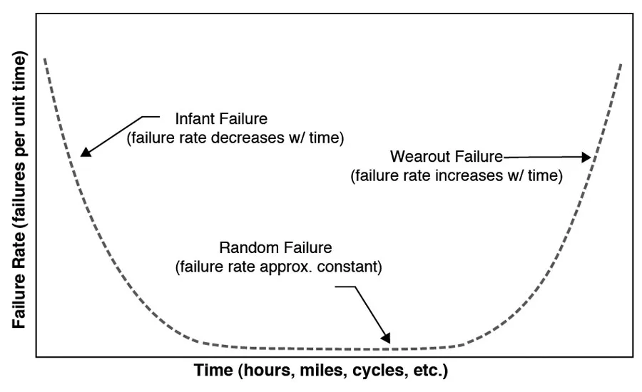
c. The Weibull plot (Figure 2) can result in life of motor falling in either of three distinct regions, often called the famous bath tub curve. If b<1 then the failures are infant failures, due to design issues, material issues or in general special reasons in design. If b= 1 then the failure rate is constant and such failures are called useful life failures or random failures. This is the life for which we mainly aim.  If b>1 the failures are wear out failures and they increase with time.

5. Calculating X and Y axis Values of Weibull Curve

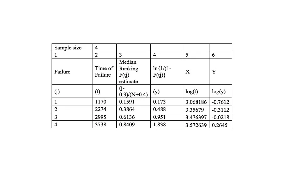
a. The Weibull curve is plotted on a log-log graph. Let us assume that we have tested four motors at one of those points as indicated in Figure 1, and that all the test units were tested to failure and their failure times were recorded.

b. The failure times t needs to be arranged in increasing order – 1170 Hrs , 2274 Hrs, 2995 Hrs, and 3738 Hrs.

c. The corresponding X-axis values in Weibull curve are simply the natural logarithm of each time to failure i.e. ^X=In(t). We can also take base 10 logarithms which are used in this case.

d. The corresponding Y-coordinate requires calculation of failure probability F(t) or the unreliability of these motors. This means, we need to come up with unreliability estimates for each of our failure times in order to plot the data on a two-dimensional Weibull plot. These unreliability estimates are calculated by median ranking (MR) using Benard’s approximation.  It has the form:

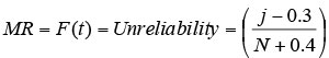
Where N is the total number of failures (in this case N = 4) and j is the failure order number. In this case j =1 for failure at 1170 Hrs, j=2 for failure at 2274 Hrs, j=3 for failure at 2995 Hrs and j=4 for failure at 2995 Hrs.

To arrive at Y axis value of Weibull curve we need to perform below steps:

• Calculate unreliability estimates F(t) for each of our failure times based on Benard’s approximation
• Use the above unreliability estimate for each failure and calculate the function

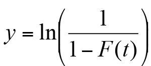
• From the value of , the Y axis coordinates of Weibull plot can be calculated taking the natural logarithm of .  We can also take base 10 logarithms which are used in this case.

The X and Y coordinates are organized in column 5 and column 6 of the table shown below.

6. Plotting Weibull Curve

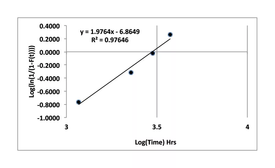
a. The next step is to use an excel spreadsheet to make a scatter plot with X axis as column 5 & Y axis as column 6 (Table 1). Then fit a line and display the equation of the line and degree of fit R2 on the plot (Figure 3)

Life Prediction Using Weibull Plot

a. Shape Parameter b(slope of  Weibull line)

The above graph gives the shape parameter bas 1.974. Since the value of bis >1 hence these failures are wear out failures.

b. Characteristics Life h

The equation of Weibull line above gives intercept on x axis b ln has -6.8649. From this we can calculate the characteristics life   by substituting value bin it. The value of characteristics life is 2975 Hrs. 

c. B10 Life

B10 life is life corresponding to 10% of failure or 90% reliability. The above two parameters can be substituted in Weibull reliability equation to calculate B10 life. The details of Weibull reliability equation and its linear formulation are placed in Appendix for reference.  In this case B10 is 950 Hrs.   

Summary

This white paper summaries the method to calculate reliability of permanent magnet brush DC motors using Weibull estimation probability plotting technique. This systematic first order approach can help an individual to study life characteristics in these motors without the help of high end statistical tools.

Appendix

Linearization of Weibull Cumulative Distribution Function

Reliability of permanent magnet electric motor depends on its application and the environment where it is used. However, manufacturers of such motors can establish their life based on a controlled set-up available at their end irrespective of the real application.

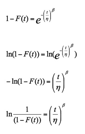
We will use famous Weibull distribution using probably plotting technique for establishing the reliability. Weibull distribution is widely used for life prediction because it’s most generic distribution and in special cases (function of data & its distribution parameters) limits to other types of distribution – normal, exponential, binomial etc. The cumulative distribution function cdf or unreliability function of the two-parameter Weibull distribution is given by:

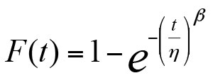
where n is called scale parameter and bis called shape parameter.

The next step is to linearize this function in the form of straight line y = mx + b:

For this we need to transfer 1 in above equation to left hand side and taking natural logarithm of this

Again taking natural logarithm of this

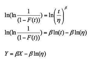
Where

This equation resembles with y = mx + b because all the variables are of the first order. This is now a linear equation, with a slope of band an intercept of ^-bln(h).

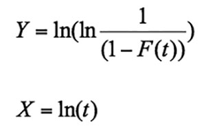
Therefore the x- and y-axes of the Weibull probability pl ot can be made. The x-axis is simply logarithmic, since ^{X = ln(t)}. The y-axis is slightly more complicated, since it must represent:

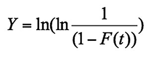
Where F(t) is the unreliability.