Production engineers often get excited about new technologies and tend to think that the benefits of investing in them are obvious to everyone else in the company. However, enthusiastic engineers can get an unpleasant surprise if they are not prepared to argue their case properly.

Whenever engineers seek to add a new technology to the shop floor, management invariably asks the same question: What is the payback period of the proposed investment? That’s a fair question, but it’s worth pointing out that “payback period” does not actually describe the profitability of an investment; it just describes the time needed to “repay” the amount of money used for the investment. It does not take into account the time value of money, the risks involved, opportunity costs, and other factors.

Therefore, the preferred tool for evaluating the profitability of equipment investments is one that uses net present value (NPV) instead of—or in addition to—the calculation of “payback time.” Internal rate of return (IRR) or calculations based on annuity can also be used.

A typical NPV formula looks like this:

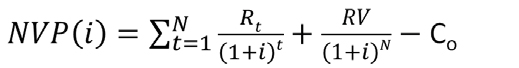
In this equation, NPV(i) is the discounted value of the investment; t is the time period (years); N is the total number of periods (depreciation time); i is the company-set target for internal rate of return; R_t is cash flow during period t; RV is residual value at the end of depreciation time; and C_o is the total initial investment cost.

If, with the given restrictions for N and i, the output NPV(i) is more than 0, the investment will be profitable.

NPV calculations are useful:

• when comparing different kinds of investments with each other, like “paint shop” vs. “welding line.”
• when making simple “apples to apples” comparisons like, “Should I purchase welding power source A or B?”
• when making “make or buy” decisions.

In these cases, the NPV will show which investment is the most profitable, as indicated by the highest NPV value. There should be one NPV value for each alternative production concept, including the current setup.

It’s important to remember that, when comparing NPV figures, we see only the relative profitability of different production concepts. Typically, shareholders seek both growth and profitability for their companies. It is essential that compared production concepts are compatible with both goals. All concepts must offer same capacity, so that cost per produced unit can be calculated with the same volumes.

Since targeted internal rate of return (i) and depreciation time (N) are more dependent on company internal financial rules and local laws than actual manufacturing operations, these factors are not addressed in this paper in detail. At any rate, they should be the same for all comparable investments.

While the residual value of nonautomated production equipment might easily be estimated as zero, the residual value of the automation investment can still be significant after the depreciation period. Depending on company policy, the depreciation time can vary a lot, but generally three to seven years should be acceptable. However, the average technical lifetime for a robot is 12 to 15 years.

Therefore, it’s fair to argue that some residual value, at the end of this relatively short depreciation time, should be taken into account when making investment calculations for automated production systems.

Initial investment cost should include the cost of the equipment, as well as software, training, project management and other internal costs, such as infrastructure changes, required by the proposed investment. These costs are related time-wise directly to purchasing and commissioning of the automation system.

Cash flow in each period can be calculated as follows:R_t = earnings – operational costs.

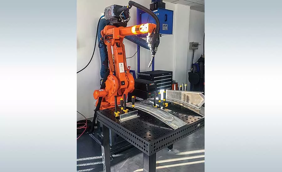
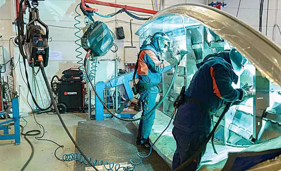
Earnings represent the net increase in customer value that the investment provides. For example, in the case of a welding robot, it can be the sales value of welded joints produced during a time period. Thus, it’s easy to see that the feasibility of an automation investment depends heavily on a high utilization rate. In the case of robotic arc welding, one robot can produce 6,000 to 12,000 kilograms of welds per year, while one manual welder can only produce 1,500 to 2,000 kilograms of welds annually. If we assume that the customer pays the same amount of money per kilogram of welded material, the earnings are easy enough to estimate for both concepts.

Direct Labor vs. Automation

When estimating the profitability of investments in production automation, one should be aware of the following points:

• Comparing only direct labor cost (dollars per hour) to the proposed investment easily leads to wrong conclusions.
• To determine the R_t factor in the NPV formula accurately, we must understand the role of manufacturing activities in company as whole.

While most companies know exactly how much hourly wages are today, they are not necessarily aware of how much each actual manufacturing function costs the company today or in the coming years.

In this article, the costs are divided into the three categories, representing cost factors that should be determined for all alternatives before any real comparison between choices can be made.

The first category represents the direct costs of production, such as wages; the floor space for each work stage; management and supervision; tools and materials; and shared utilities, such as overhead cranes.

The second category represents costs that actually burden the work stage, but are harder to define if they have not been systematically traced. They occur, for example, because of the current way operations are done. These costs could be related to quality activities (inspection or repair work); work in progress (WIP); long or varying lead times; health and safety; overtime or additional working hours in downstream areas that are needed to manage variability of manual work in previous stages; and additional working hours for supporting resources, like supervision and logistics. Sometimes, the cost of reduced WIP alone can justify the investment on automation!

The third category is costs related to the availability of resources over a period of time. They are rarely calculated accurately, but only estimated. Here are a few examples:

The easiest to understand here are the costs for skilled labor, which are increasing because of macroeconomic reasons. One company has little or no means at all to influence these. Since investments on production automation are made for several years in the future, the labor costs of today cannot be used for the total period of an investment’s life time. Instead, the changes in labor costs over a period of 10 to 15 years should be taken into account. A 7 to 15 percent annual rise in these costs is not unheard of.

The effect of learning curves can be decisive. Each time a new product is introduced to the line, the processing time for the first unit can be 50 to 150 percent longer than the calculated optimum target time. It takes several products for workers to learn how to achieve the target throughput time. Automation standardizes production activities, because once it’s set up, it repeats the same activity ever after—unlike people. This can result in dramatic savings in lead times with every new product introduction.

The last point is not an actual cost factor, but a fundamental fact to be recognized: Can the job be done without automation? Can the targets for production volume and profit be reached when considering accuracy, quality, speed, the health and safety of workers, the general availability of skilled workers, and limitations on floor space, storage space and material flow.

If the conclusion is that the job cannot be done without automation, then using labor cost as a basis for comparison and as an element in ROI calculations is more or less irrelevant.

Key Performance Indicators

Once the all cost factors are identified, they can be added up and tied with actual products rather than resource hours. At this point, simple key performance indicators (KPI) can be made available for production stages. These could be the cost of produced steel (dollars per ton); the cost per weld (dollars per meter or kilogram of welded material); the cost of average WIP (dollars); and the inventory turnover rate.

Current KPI figures can be compared with estimated KPI figures based on the investment. The new production concept should be able to give better results, over the chosen time frame, as visualized by selected KPIs than the existing system. Similarly, in case of “green field” factories, two or more different concepts can be compared.

Apples and Oranges

To understand the impact of investments in automation, a wider perspective should be taken. Any investment in new machinery will involve more than just the equipment itself. Production planning and scheduling may need to be modified for the new production concept.

Investments on automation should be considered as a strategic issue, and your entire production concept should be evaluated instead of individual work steps. Traditional investment calculation tools can be used to evaluate the profitability of automation investments, if a comprehensive and compatible evaluation of alternatives is done. The key question is then which concept provides the best profitability and production capacity for the company? “What is the cost per produced unit over a specific period of time?” is a more relevant question than, “How much does this one piece of equipment cost?”