Screwdriving and Riveting
Robots Automate Bolt-Tightening on Automotive Assembly Lines
3D vision sensors are a key enabling technology.
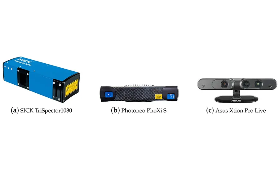
The researchers evaluates three sensors: the Sick TriSpector1030 (laser line triangulation), the Photoneo PhoXi S (visible stripe pattern structured light) and the Asus Xtion Pro Live.
Tightening bolts with a six-axis robot was once thought impossible. The robot simply could not match the precision, dexterity and feel of a person with a handheld tool.
Today, that’s changing. Using 3D vision systems and force sensors, robots can tighten bolts on assemblies even under the demanding conditions of a car factory.
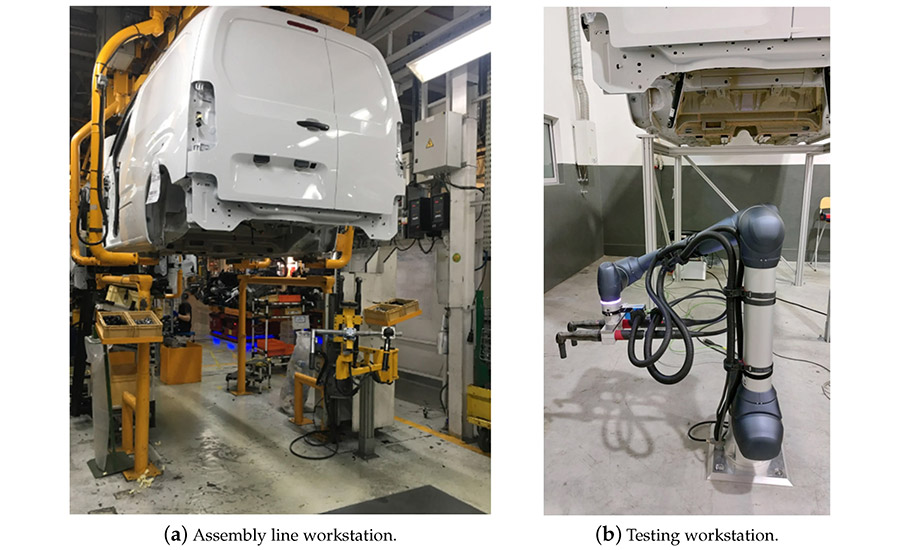
These images show the workstations on the assembly line and the testing environment for fastening the two rear axle dampers. Source: Institute for Systems and Computer Engineering, Technology and Science
3D vision is ideal for this application because it is less sensitive to ambient lighting conditions and dirt. The capabilities of this technology have increased markedly in recent years. The systems are more compact, have greater processing capacity, and offer more advanced image-processing algorithms.
Given the importance of this technology to this application, we set out to compare several 3D vision systems to determine which one is best for automating fastening on an automotive assembly line.
Specifically, we looked at the process of fastening rear axle dampers to the undercarriage of a van. The vans are transported from station to station on an overhead conveyor. When a van arrives at the workstation, an assembler picks an axle damper from a bin, goes underneath the vehicle, and installs it to the rear undercarriage, which has two attachment points.
Next, the assembler hand-starts two bolts at those points. Then, using a pair of fixtured electric tools, the assembler tightens both bolts at once. This process is performed for both the left and right rear wheels.
Since this task is repetitive and non-ergonomic, the automaker wanted to automate the process. Now, the assembler still installs the dampers, but a vision-guided robot tightens the bolts.
Looking for quick answers on assembly and manufacturing topics? Try Ask ASM, our new smart AI search tool. Ask ASM
Since the position of the van at this workstation varies due to mechanical tolerances of the conveyor and the weight of the vehicle, the robot must perceive the position of the axle damper attachment structure to successfully perform the bolt-tightening operation. So, 3D vision is critical for this application.
In addition to comparing sensors, we assess the success of our robotic bolt-tightening system. Unlike other approaches, which depend solely on the vision system’s ability to find the bolts themselves, our system relies on the 3D perception of the structure of the vehicle in which the bolts were attached. This approach allows for unambiguous pose estimation in six degrees of freedom, as the vehicle’s structure has a surface with unique geometry and a higher number of points compared to the bolts.
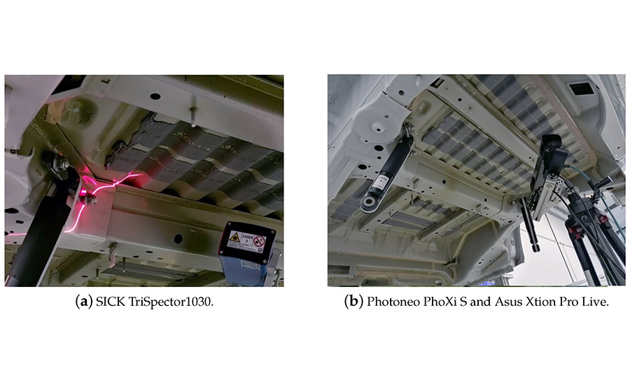
These images show the 3D sensors in place for capturing measurements. Source: Institute for Systems and Computer Engineering, Technology and Science
3D Sensing Technologies
3D sensors can be classified as active or passive. Passive sensors, such as stereo cameras, rely on the light reflected from external sources for observing the environment. Active sensors rely on their own source of radiation for probing the environment, making them more robust for scanning textureless surfaces and dark environments. Examples of active sensing technologies include laser triangulation, structured light, and time of flight.
One of the most reliable and accurate optical sensing technologies is laser triangulation (point or line). The resulting 3D point cloud is computed by interpreting the deformation of the laser line when observed from the camera perspective. Coupled with a known movement of the object on a conveyor or the sensor mounted on a track or robotic arm, several 3D scan profiles can be merged to form a 3D point cloud of the surface.
These sensors are usually small and have a high acquisition rate (1 kilohertz). The biggest disadvantage of this technology is the requirement to generate a known movement, either of the object or of the sensor itself. Despite this, 3D laser triangulation is often chosen because it provides greater robustness to variations in ambient light and the materials.
Structured light sensors are widely used in industry for 3D perception and inspection, given their high accuracy, high density point cloud and robustness for scanning textureless surfaces.
They consist of a light projector and one or more cameras. The light source projects a set of known patterns into the environment, which are distorted when they hit the surface of objects. Depending on the pattern, one or more images must be captured. For example, a speckle pattern is static and needs only one image-capture to generate sparse depth information, which can be coupled with measurement interpolations to increase the point cloud density.
On the other hand, sequential stripe patterns can achieve dense surface measurements with much higher point cloud density. But, they require several image captures with a static environment, one for each pattern with decreasing stripe thickness.
Time-of-flight cameras rely on infrared light pulses for probing the environment. They estimate the distance to objects by measuring the time difference between the pulse emission and the detection of the reflected signal. Interest in these sensors has been increasing due to their use in autonomous vehicles. Typically, these sensors produce less accurate 3D data compared with structured light sensors, and they generate more shadowed or veiled points on the border of objects. On the plus side, they have a much higher data acquisition rate.
Stereo vision systems can perform 3D reconstruction of the scene by calculating the correspondence between pixels of two different images taken by cameras in different perspectives using triangulation. Since the accuracy of 3D measurements depends heavily on identifying and correctly matching points between images from different cameras, some stereo vision systems project a pattern into the environment to refine point matching. This approach significantly improves the measurement accuracy in low-texture environments.
However, the consistency of the measurements is not as reliable as other 3D technologies. Moreover, passive stereo systems have higher measurement errors when operating in low-light environments. As a result, these sensors are used less in industrial applications.
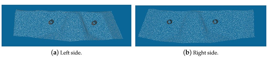
These images show the point clouds extracted from the van’s CAD file (without the axle damper) for each side of the van. Source: Institute for Systems and Computer Engineering, Technology and Science
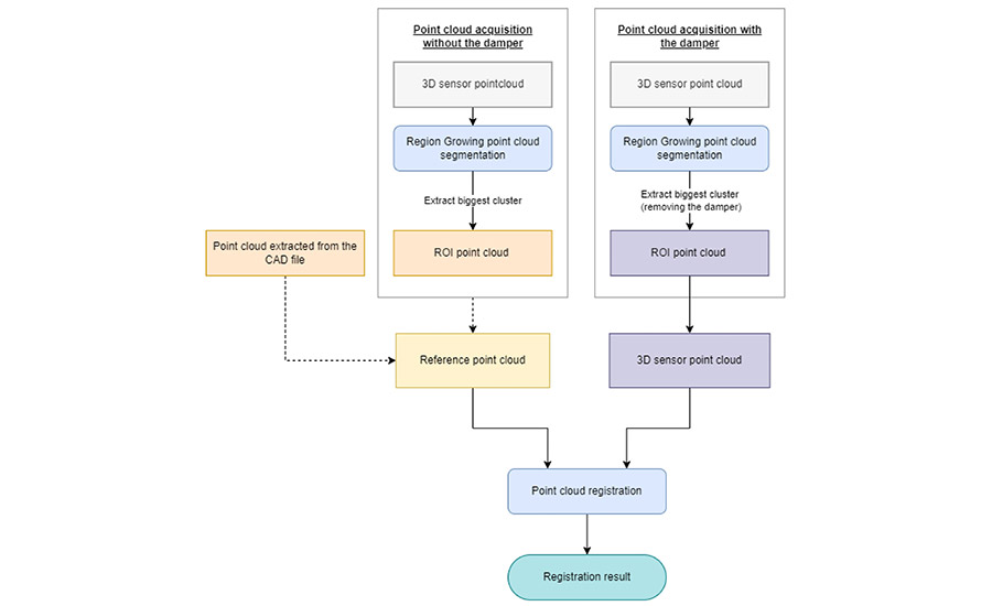
This diagram shows the methodology the researchers used for comparing the sensors. Source: Institute for Systems and Computer Engineering, Technology and Science
Comparing 3D Sensors
For our application, we had to determine the position of the axle damper attachment structure in six degrees of freedom with an accuracy of less than 3 millimeters. The surface of the part does not have texture and is painted with partially reflective white color. Moreover, the sensor would be operating without controlled light conditions. It also had to be compact, so it could be mounted on the robot arm.
With this in mind, we chose three sensors to evaluate: the Sick TriSpector1030 (laser line triangulation), the Photoneo PhoXi S (visible stripe pattern structured light) and the Asus Xtion Pro Live (infrared speckle pattern structured light).
The Sick sensor is the only one with embedded processing. It is programmed using SOPAS Engineering Tool software. The Photoneo and Asus sensors need an external PC to process their data. To compare the sensors fairly, then, we did not use the embedded capabilities of the Sick sensor, and an external PC was used to process the 3D data from all three sensors.
To compare the performance of the three sensors, point clouds of the axle damper attachment structure with and without the axle damper were acquired in a testing environment similar to the real assembly line—namely, with a real van and axle damper samples that could be manually placed and removed.
The structured light sensors were mounted on a tripod since they need to be static during the scanning procedure. The same does not apply to the laser line triangulation sensor, which was installed on the end effector of a robotic arm to capture the 3D profiles of the region of interest.
To create a data set for sensor evaluation, 12 scans were captured for both sides of the van with each sensor.
It is important to mention that in our test workstation, the van was fixed to a rigid structure and not an aerial conveyor. Therefore, to simulate the aerial conveyor deviations on the van positioning, the sensor’s poses were slightly changed manually prior to scanning.
Two reference point clouds were used as the ground truth: one extracted from the scans without the axle dampers and another from the CAD model of the van.
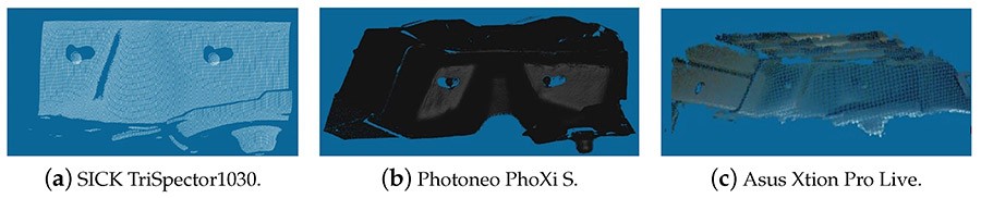
These images show the point clouds of the axle damper attachment structure without the damper. Source: Institute for Systems and Computer Engineering, Technology and Science
To create the reference point cloud from the 3D sensors scans, the point cloud without the axle dampers was filtered and segmented with the following steps:
- Scan the van without the axle damper.
- Crop the point cloud if necessary (only applicable for the Asus Xtion Pro Live sensor due to its higher scan volume).
- Segment the point cloud into clusters using the region growing segmentation algorithm.
- Extract the region of interest where the axle damper will be placed (considering the acquired point clouds, this corresponds to the biggest cluster).
The region-growing segmentation algorithm starts by sorting the points by their curvature. It then selects as the first seed the point with the lowest curvature. Then, it keeps expanding the current cluster seeds by adding neighboring points that have an angle between the current seed and the neighboring point below a given threshold. After no more points can be added to the current cluster, a new cluster is initialized with a seed point that has the lowest curvature from the points that do not yet belong to a cluster. The algorithm for growing and creating new clusters keeps repeating until all the points are associated with a labeled cluster.
This segmentation algorithm was selected because the van support structure has a locally smooth surface with transition zones to the axle damper surfaces with large curvature differences. Moreover, the support structure has a surface area that is much higher compared with the axle damper, allowing the segmentation selector to pick the cluster with the largest number of points.
After this procedure was executed for all the reference point clouds without the axle damper, the point clouds acquired with the axle damper were filtered by following the same steps.
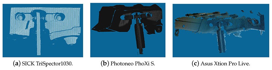
These images show the point clouds of the axle damper attachment structure with the axle damper in place. Source: Institute for Systems and Computer Engineering, Technology and Science
Then, the registration of both point clouds was performed with different voxel grids (1 and 5 millimeters). The accuracy of the point cloud registration using the iterative closest point (ICP) algorithm was measured by computing the root mean square error (RMSE), which was obtained by computing the Euclidean distance between corresponding points from the scan and reference point clouds. The RMSE was calculated for each registration, in which points with a corresponding reference point distance lower than a given threshold were marked as inliers.
The ICP algorithm aligns the sensor data with the reference point cloud by iteratively computing the six-degree-of-freedom matrix transformation that minimizes the RMSE of a given set of correspondences. For each iteration, every point in the sensor data is matched with the respective closest point in the reference point cloud. Points that have a correspondence distance higher than a given threshold are discarded from the list of correspondences to allow the algorithm to tolerate outliers.
Then, the singular value decomposition (SVD) method is used to compute the six-degree-of-freedom transformation that minimizes the RMSE of the correspondence distances. The algorithm stops when the RMSE is below a given threshold or when the computed matrix has converged and stabilized.
Our data show that the alignment results were better when using reference point clouds based on a previous scan performed by the respective sensor instead of using CAD models. This was expected, since the production of the van structure deviates somewhat from the CAD model. Moreover, registering a new point cloud with a previously captured and filtered scan can be used to evaluate the repeatability of both the sensor and the alignment algorithms.
On the other hand, the RMSE difference when comparing the usage of a reference point cloud using CAD models or scans is less significant when using a bigger voxel grid (5 millimeters) since the voxel grid replaces all the points within a cell with their mean XYZ value. This can result in the absorption of the van structure production tolerances and the sensor measurements noise, but it can also raise the mean RMSE if the reference and scan voxel grids do not have overlapping coordinate systems, resulting in an offset between the cells that grows as the voxel size increases.
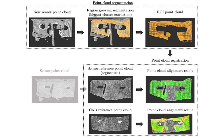
These images show the process of segmenting and registering the point clouds. Source: Institute for Systems and Computer Engineering, Technology and Science
Focusing solely on the results when using the sensor-based reference point cloud and the voxel grid of 1 millimeter, the difference between the RMSEs of the point clouds captured by each sensor is clearer. Namely, the lower RMSEs were 0.25, 0.49 and 1.01 millimeter when using the Sick, Photoneo and Asus sensors, respectively. Additionally, the percentages of inliers were 99, 92 and 88 percent, respectively. Moreover, no significant difference was found when varying the maximum inlier distance.
The difference between sensors was lower when using a voxel grid of 5 millimeters. The RMSE was 1.3, 1.4 and 1.49 millimeter, with a maximum inlier distance of 2 millimeter when using the Sick, Photoneo and Asus sensors, respectively. In this case, there were significant differences when varying the maximum inlier distance. The RMSE decreases with a smaller maximum inlier distance; however, the percentage of inliers decreases as well. Although the RMSE was smaller, the value refers to a smaller number of corresponding points.
The depth error of the SICK sensor is smaller than the other two sensors, and this specification is reflected in these results. This sensor provides the best alignment results when using both types of reference point clouds and when varying the voxel grid and the maximum inlier distance. Considering the voxel grid of 1 millimeter, the RMSE was always below 1 millimeter with the percentage of inliers above 85 percent, even when using the CAD point cloud as the reference model. The RMSE increased above 1 millimeter when changing the voxel grid for 5 millimeter, but, overall, the SICK sensor performed better than the other sensors.
We were also able to achieve an RMSE of around 0.5 millimeter with the Photoneo sensor using a sensor-based reference point cloud with a voxel grid of 1 millimeter. Overall, the Photoneo performed worse than the Sick, but better than the Asus. In general, the Asus generated the worse results, with an RMSE always above 1 millimeter. This was related to the lower quality of the captured point cloud, which had less accuracy and higher sensor noise.
The lower RMSE achieved by the Sick sensor was likely due to the usage of camera lens filters that block all light except for light the frequencies associated with the laser line. This way, the sensor will have better repeatability, since the camera sensor will have less pixel noise when compared with the other two sensors, which capture light from a much wider frequency range. On the other hand, by being a line triangulation system, Sick can also employ subpixel algorithms to estimate the center of the detected laser line, further increasing its precision and repeatability.
The time needed to process the registration and pose estimation was lower when using the bigger voxel grid (5 millimeters), since the point cloud was less dense.
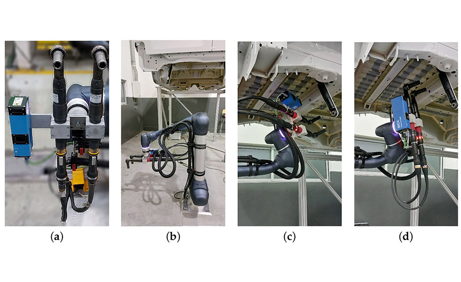
Our workstation consists of a six-axis cobot with a reach of 1,700 millimeters and a maximum payload of 20 kilograms. Two screwdrivers are attached to the cobot’s end-effector. Source: Institute for Systems and Computer Engineering, Technology and Science
Machine Vision for Fastening Operations
Given the test results, we chose the Sick sensor for our robotic fastening station. Our six-axis cobot had a reach of 1,700 millimeters and a maximum payload of 20 kilograms. Two screwdrivers were attached to the cobot’s end-efffector. The robot base was centered in relation to the left and right axle damper locations.
The process works as follows:
- The robot moves the 3D sensor to scan the van without the axle damper to create a reference point cloud.
- The pose of the attachment structure with respect to the robot is determined.
- The assembler places the axle dampers in position on the van.
- The robot moves the sensor to capture a new scan of the van with the axle damper in place.
- The new point cloud is aligned with the reference point cloud using the ICP algorithm.
- The point cloud alignment is validated to ensure that it has a minimum percentage of overlap between the reference point cloud and the new scan.
- The transformation matrix between the robot base and the axle damper attachment structure is computed.
- The robot tightens the bolts.
The total cycle time is 160 seconds.
Editor’s note: This article is a summary of a research paper co-authored by Joana Dias, Carlos M. Costa, Germano Veiga and Luís F. Rocha of the Institute for Systems and Computer Engineering, Technology and Science; and Pedro Simões and Nuno Soares of Europneumaq Industrial Solutions in Serzedo, Portugal. To read the entire paper, click here.
For more information on robotic screwdriving, visit www.assemblymag.com to read these articles:
Looking for a reprint of this article?
From high-res PDFs to custom plaques, order your copy today!