Electronics Assembly
Thermal-Cycle Life Tests of Solder Joints in Electronic Assemblies
A variety of environmental stress factors--such as temperature and humidity, thermal and functional cycles, corrosion, shock and vibration, handling, shipping and reworking--may lead to solder joint failures in electronic assemblies. Therefore, product development often requires solder joint thermal-cycle life testing. Testing involves periodic inspection of samples under extreme environmental conditions. However, prototypes, facilities and inspections are expensive, and running tests is time-consuming. Therefore, how do test engineers get as much information as possible in a timely manner? To do so, they must decide how many samples to test, how often to inspect them, and whether the test can be stopped before all samples have failed. They must also pick a method of analysis.
This article discusses the thermal-cycle life tests of solder joints in electronic assemblies. Although it specifically discusses solder joints, the statistical methods could apply to life testing of any assembly.
What's a Useful Metric?
Two types of testing methods are common. The pass-fail test is the simplest. It asks whether the samples passed or failed a specific threshold.Pass-fail tests are not as simple as one might think, and they certainly don't describe the population. For borderline populations, sample-size selection can be a very important factor. In fact, it could prove that a borderline population passes by testing only a few samples.
A second testing method describes the distribution of failure times of the underlying population. This test method is used to compare one product vs. another, check process stability or product uniformity, quantify a material change or provide expected failure rates. This testing method, though, needs a good metric (i.e., deciding information).
The first thing to remember is that swooping, full-color curves are pretentious, probably inappropriate and impractical for decision-making. Instead, report a metric showing when most samples fail, along with a metric that indicates the breadth of distribution.
For life testing, the median or F50 is a good central metric. This is simply when 50 percent of the sample population fails. Another option is the Weibull "eta," which is when 63 percent fails. However, most testing engineers prefer using 50 percent.
The next necessary metric must indicate breadth. Using F1, along with F50, to derive this figure is best. F1 is when 1 percent of the sample population fails. The ratio of F50 to F1 defines the slope and enables plotting a straight Weibull-log line. Anyone can derive any desired value from this. An undesirable alternate is the Weibull "beta," which is an arcane Weibull breadth indicator. This breadth indicator cannot be plotted and is useless in practice.
Measuring the Goodness of a Metric
The quality of your results is determined long before the data start coming in. Quality is built into the test plan. It is not determined or discovered after the test. Therefore, it is not wise to wait for after-the-fact analysis. The best testing methods are arranged with perceived data quality already in mind.Quality can be defined as how well the metric describes the underlying population. Given that, the selection of testing factors will determine the quality of the resulting metrics. Tests can generate ballpark values, or they can discriminate between similar populations. Solid numerical measures of goodness are available for making these decisions. But what is a proper measure of goodness?
Looking for quick answers on assembly and manufacturing topics? Try Ask ASM, our new smart AI search tool. Ask ASM
Statistics offers a useful measure of goodness--the confidence interval (CI). This is a calculated function of the breadth of the population and the number of samples. Good software will automatically provide the CI. A small CI is good. It indicates confidence that the underlying population metric is within a small interval. A large CI means that only the population metric is somewhere within a large interval.
The CI is also useful to decide whether one population is really different from another. If the CIs do not overlap, the samples are different. If the CIs do overlap, the samples are likely to be from the same population and are likely to be identical.
How Do We Design the Test?
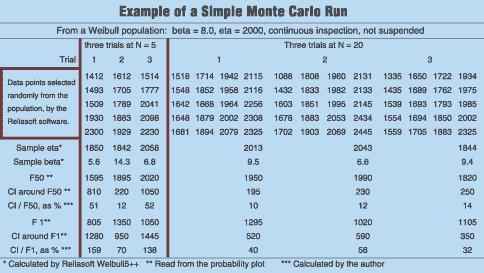
The best way to learn about something is to try it. Statistics refers to this as the Monte Carlo method. The Monte Carlo method lets you see the quality of metrics to come, before you see any hardware or data.
To study a particular distribution, random samples from the population are selected and then analyzed under a set of conditions to see what uncertainty is acquired. This is done several times for different distributions, sample sizes, inspection frequencies or suspensions. You will begin to determine the effect of each test variable on the resultant uncertainty. The following is an example. If you have a population and you want to know what sample size is needed to describe the F50 of that population, you would first select the distribution you're interested in. Draw a sample set N=5 and calculate F50. Draw another five and calculate F50. Do this many times. You will discover that the F50s vary widely and will have large CIs. Now draw several N=20 sets and calculate F50s. The resulting F50s will be nearly identical, and the CIs will be small. By using Monte Carlo analysis, you have demonstrated that a larger sample size provides a more accurate measure of the population.
Effect of Inspection Frequency
Inspection frequency is important. Typically, samples are inspected periodically. However, situations often occur where a sample failed between X and Y cycles, but the exact time is unknown. This can lead to concerns that infrequent inspections will jeopardize quality. However, when properly treated, this sort of data can be good, even if you have as few as four to six inspections during the population's failure span. Also, inspection intervals don't need to be the same throughout the test.Suspending a test when 60 to 80 percent of samples have failed can save time and money, without serious quality penalties. To take full advantage of this, a large sample size and high inspection frequency are important. Good software or manual methods are also necessary.
The benefit in time-savings can be significant. In an eta=2,000, beta=8 test, approximately 2,000 cycles can be saved by suspending testing at 60 percent. At 15 cycles per day, that is equivalent to 4 months.
Effect of Distribution of the Data
Failure distributions can be broad or narrow. Tightly controlled solder-joint populations fail in a narrow distribution (Weibull beta=8 to 12). Sloppier control or several overlapping failure modes will result in a broad distribution (beta=2 to 4), or log-normal or bimodal distribution. If your sample size numbers 50 or less, you cannot tell by looking at the straightness of a line of plotted points whether the population is Weibull or log-normal.
In this case, Weibull is best, unless you are sure that all your data are log-normal. The uncertainty of any metric, at any sample size, will always be better in a narrow distribution compared to a broad one. From a narrow distribution, any sample is going to be close to the other samples, so it doesn't matter how many you test. Tailor your test plan to fit your expected distribution.
Data-Reduction Methods
Manual methods of data reduction can be effective. Plot each continuous-data failure point and run a best-fit straight line. Then read off the F50 and F1. For N=10, your metrics will be within approximately 10 percent of what you'd get from good software. For N=20+, any difference in F50 estimates is trivial. However, for N=5, the F50 will be 15 to 25 percent off, and the F1 will be a bit worse. The small sample size is the problem, not the method. Suspended data, plotted properly manually, will closely match software's straight-line curve fit. Intervalized data can also be manually plotted and will match software results. However, it is essential to find the failure point between the time it was ok and the next time that it failed. If several fail within that interval, spread out the failures uniformly within the interval. This is a bias-free method. It is mathematically and logically incorrect to graph points at the end of the interval. Attempting to manually calculate the CI will probably be futile. The conclusion regarding the adequacy of manual graphing can be demonstrated in a few minutes using Monte Carlo trials with good software.Metrics in Literature
Typical tests that are reported in various sources are often statistically imprecise. These metrics can be evaluated by estimating the CIs, but only if actual data is presented. Unfortunately, that data is usually not reported.In a hypothetical case, where beta is six, eta is 1,000 and inspections occur every 100 cycles, Monte Carlo analysis demonstrates that the F50 uncertainty will be 47 percent and the F10 uncertainty will be 82 percent. Even worse, when you see a sample size of five, assume any midrange metric will be at least 200 percent off. However, with a sample size of 30 or more and a tight beta (eight to 12), some persuasive evidence of frequent or continuous inspection, no suspension and proper data reduction, you can be 95 percent confident that the F50 will be within 5 percent of the true population F50.
If only a line on a graph is shown and there are no data points, assume there is a reason. Fully reported data can be analyzed to determine its uncertainty.
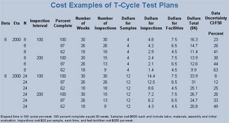
Cost Impact
Samples, inspections and time cost money. But what do you do when you need a certain level of quality of your resulting metrics? Treat this decision just like any other business or engineering decision. Do some tests or trade-off studies. If you know your costs, you can anticipate the sort of failure distributions (Weibull beta and eta) that will be encountered. Life tests can be treated like any other task, using comfortable principles and tools. Good software and Monte Carlo analysis can help you plan an optimum test, and can help you evaluate the life test data.Looking for a reprint of this article?
From high-res PDFs to custom plaques, order your copy today!